
SPC DEMO
Don’t miss out! Book a demo of our specialized SPC software and unlock immediate improvements in your processes.
SPC DEMO
Don’t miss out! Book a demo of our specialized SPC software and unlock immediate improvements in your processes.
Attributes step-by-step interpretation
You do not have enough data to get good estimates of process spread and location. For a more accurate picture of your process, you should have at least 100 data values or 20-25 subgroups (samples).
SPC DEMO
Don’t miss out! Book a demo of our specialized SPC software and unlock immediate improvements in your processes.
SPC DEMO
Don’t miss out! Book a demo of our specialized SPC software and unlock immediate improvements in your processes.
SPC DEMO
Don’t miss out! Book a demo of our specialized SPC software and unlock immediate improvements in your processes.
Quality Advisor
A free online reference for statistical process control, process capability analysis, measurement systems analysis,
control chart interpretation, and other quality metrics.
SPC DEMO
Don’t miss out! Book a demo of our specialized SPC software and unlock immediate improvements in your processes.
7. Analyze the results
The completed analysis for the example is shown below.
Calculations:
|
|
|
|
Zupper = 2.00
|
Zlower = 5.00
|
|
Cpk = 0.67
|
Cp = 1.17
|
|
Cpu = 0.67
|
Cpl = 1.67
|
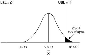
Examine the capability indices and the distribution. What do they show? Is the process capable? In the example, the process is off center, reflecting a capability issue. The upper specification of 14 minutes cannot be achieved consistently. The team must either improve the process or revise the specification. In the example, the team chose to revise the specification, but this is not an option in many industries.
The aim of capability is to achieve improved Cpk values, resulting in a more capable system. For most industries, the aim is to achieve a Cpk of at least one. Certainly this is the case for most service organizations. Some manufacturing companies require Cpk values greater than one. For example, the minimum is frequently 1.33, providing room for process drift, etc. When parts are being assembled, reduced variation at the center of the specification gives considerable benefit, namely parts assemble more quickly and more easily. Motorola, for example, constantly strives for higher and higher Cpk values. The company’s 6-sigma program has received a great deal of attention, and translates to a Cpk of 2.0. By pushing for improved Cpk values, the improvement effort is focused on shrinking variation around the center of the specifications.
Caution: If a process is unstable—that is, if special causes are evident in the control chart—capability analysis will be unreliable. Every time the capability indices are calculated, they will be different. Special causes should be removed from a process. While special causes are present, the process is unpredictable, causing it to go in and out of specification. As soon as a special cause occurs, the Cpk is meaningless, since special causes often result in unpredictable defects; even an apparently good Cpk can not be relied upon.
If the sampling selected in the control chart is not appropriate for the process, this can also affect the Cp/Cpk values. For example, sampling too frequently will artificially reduce the range values and cause the Cp/Cpk values to appear high. Using the wrong sample size can have a similar effect. Refer to the sampling section for guidance with appropriate sample size and frequency.
If the data being analyzed is not normal, the estimated standard deviation () will not be accurate. Nonnormal capability analysis must be used if the distribution is not normal, refer to the topic “Nonnormal capability analysis,” later in this section for more information. The method shown in this section can be significantly affected by non-normal data, giving inaccurate results.
The above article is an excerpt from the “Operational definition” chapter of Practical Tools for Continuous Improvement Volume 2 Statistical Tools.
Quality Advisor
A free online reference for statistical process control, process capability analysis, measurement systems analysis,
control chart interpretation, and other quality metrics.
SPC DEMO
Don’t miss out! Book a demo of our specialized SPC software and unlock immediate improvements in your processes.
6. Calculate and interpret the capability indices
This step describes the key capability indices.
>> 6.1. Calculate Cp
>> 6.2. Calculate Cpk
>> 6.3. Interpret Cp and Cpk
>> 6.4. Calculate Cpu and Cpl
The above article is an excerpt from the “Operational definition” chapter of Practical Tools for Continuous Improvement Volume 2 Statistical Tools.
Quality Advisor
A free online reference for statistical process control, process capability analysis, measurement systems analysis,
control chart interpretation, and other quality metrics.
SPC DEMO
Don’t miss out! Book a demo of our specialized SPC software and unlock immediate improvements in your processes.
6.4. Calculate Cpu and Cpl
Cpu and Cpl are the Cpk values calculated for both Z values.
Therefore, Cpu is:
For the example:
Cpl is:
For the example:
From Cpu and Cpl, it is evident that the smaller value for the example is Cpu, which is the same value as Cpk. By comparing Cpu to Cpl, it is evident that the overall average is off center and closer to the upper specification than the lower specification. The larger the difference between the Cpu and Cpl, the more off center the process.
The above article is an excerpt from the “Operational definition” chapter of Practical Tools for Continuous Improvement Volume 2 Statistical Tools.
Quality Advisor
A free online reference for statistical process control, process capability analysis, measurement systems analysis,
control chart interpretation, and other quality metrics.
SPC DEMO
Don’t miss out! Book a demo of our specialized SPC software and unlock immediate improvements in your processes.
6.3. Interpret Cp and Cpk
The Cp and Cpk indices are the primary capability indices. Cp shows whether the distribution can potentially fit inside the specification, while Cpk shows whether the overall average is centrally located. If the overall average is in the center of the specification, the Cp and Cpk values will be the same. If the Cp and Cpk values are different, the overall average is not centrally located. The larger the difference in the values, the more offset the overall average. This concept is shown graphically below.
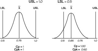
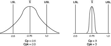
Cpk can never exceed Cp, so Cp can be seen as the potential Cpk if the overall average is centrally set. In the example, Cp is 1.17 and Cpk is 0.67. This shows that the distribution can potentially fit within the specification. However, the overall average is currently off center. The Cpk value does not state whether the overall average is offset on the upper or lower side. It is necessary to go to the Z values to discern this. An alternative is to show the capability indices Cpu and Cpl.
The above article is an excerpt from the “Operational definition” chapter of Practical Tools for Continuous Improvement Volume 2 Statistical Tools.